Active Learning

The class provides tools for active learning of regression models using expected model change (EMC) and query by committee (QBC) methods and approaches for distribution shift alleviations.

The central idea behind any active learning approach is to achieve lower prediction errors (higher accuracy) in machine learning models by choosing less but more informative data points.

The implementation of this algorithm follows an interactive approach. In other words, we often ask you to provide labels for the selected data points.

Here is a list of main methods to carry out an active learning approach:

initialize
deposit
ignore
search
visualize

[1]:

import warnings
warnings.filterwarnings('ignore')

from chemml.optimization import ActiveLearning
from chemml.datasets import load_organic_density
import numpy as np
import pandas as pd

For this tutorial, we load a sample data from ChemML datasets.

[2]:

smi, density, features = load_organic_density()
print('labels  : density,    ', type(density), ', shape:', density.shape)
print('features: molecular descriptors,', type(features), ', shape:', features.shape)

labels  : density,     <class 'pandas.core.frame.DataFrame'> , shape: (500, 1)
features: molecular descriptors, <class 'pandas.core.frame.DataFrame'> , shape: (500, 200)

Keras model example

The current version of the EMC approach only work with Keras deep learning models. You should create a function that returns a Keras model. You can also set the optimizer parameters and compile the model inside the function. Here is a toy example for the Keras model:

[3]:

from keras.layers import Input, Dense, Concatenate
from keras.models import Sequential, Model
from keras.optimizers import Adam
from keras.callbacks import EarlyStopping
from keras.initializers import glorot_uniform
from keras import regularizers
from keras import losses
from keras import backend as K

[4]:

def model_creator(nneurons=features.shape[1], activation=['relu','tanh'], lr = 0.001):
    # branch 1
    b1_in = Input(shape=(nneurons, ), name='inp1')
    l1 = Dense(12, name='l1', activation=activation[0])(b1_in)
    b1_l1 = Dense(6, name='b1_l1', activation=activation[0])(l1)
    b1_l2 = Dense(3, name='b1_l2', activation=activation[0])(b1_l1)
    # branch 2
    b2_l1 = Dense(16, name='b2_l1', activation=activation[1])(l1)
    b2_l2 = Dense(8, name='b2_l2', activation=activation[1])(b2_l1)
    # merge branches
    merged = Concatenate(name='merged')([b1_l2, b2_l2])
    # linear output
    out = Dense(1, name='outp', activation='linear')(merged)
    ###
    model = Model(inputs = b1_in, outputs = out)
    adam = Adam(lr=lr, beta_1=0.9, beta_2=0.999, epsilon=1e-8, decay=0.0)
    model.compile(optimizer = adam,
                  loss = 'mean_squared_error',
                  metrics=['mean_absolute_error'])
    return model

[5]:

m = model_creator()
m.summary()

Model: "model"
__________________________________________________________________________________________________
Layer (type)                    Output Shape         Param #     Connected to
==================================================================================================
inp1 (InputLayer)               [(None, 200)]        0
__________________________________________________________________________________________________
l1 (Dense)                      (None, 12)           2412        inp1[0][0]
__________________________________________________________________________________________________
b1_l1 (Dense)                   (None, 6)            78          l1[0][0]
__________________________________________________________________________________________________
b2_l1 (Dense)                   (None, 16)           208         l1[0][0]
__________________________________________________________________________________________________
b1_l2 (Dense)                   (None, 3)            21          b1_l1[0][0]
__________________________________________________________________________________________________
b2_l2 (Dense)                   (None, 8)            136         b2_l1[0][0]
__________________________________________________________________________________________________
merged (Concatenate)            (None, 11)           0           b1_l2[0][0]
                                                                 b2_l2[0][0]
__________________________________________________________________________________________________
outp (Dense)                    (None, 1)            12          merged[0][0]
==================================================================================================
Total params: 2,867
Trainable params: 2,867
Non-trainable params: 0
__________________________________________________________________________________________________

To view workflow, you need to install pydot. For example with pip install pydot. Then run the following code

[6]:

from IPython.display import SVG
from keras.utils.vis_utils import model_to_dot

SVG(model_to_dot(m).create(prog='dot', format='svg'))

[6]:

../_images/ipython_notebooks_active_model_based_9_0.svg

Initialize active learning: EMC

You first need to instantiate the active learning class using the model_creator function and the pool of candidates (i.e., U) represented by your choice of features.

[7]:

al = ActiveLearning(
           model_creator = model_creator,
           U = features,
           target_layer = ['b1_l2', 'b2_l2'], # we could also enter 'merged' layer because it only does the concatenation
           train_size = 50,  # 50 initial training data will be selected randomly
           test_size = 50,  # 50 independent test data will be selected randomly for the entire search
           batch_size = [20,0,0] # at each round of AL, labels for 20 candidates will be queried using EMC method
           )

you first need to initialize the method to get the indices for the training and test data:

[8]:

tr_ind, te_ind = al.initialize()

The array of queried points are always available via the queries attribute

[9]:

al.queries

[9]:

[['initial training set',
  array([445, 171, 373, 342, 372,  99, 331, 195, 199, 130, 140, 201, 451,
         300, 294, 108, 369,  79, 328, 398, 485, 426,  43, 391,  71, 124,
         495, 276, 316, 383, 498, 225, 440, 148, 122,  35, 178, 456, 253,
         216, 131, 374, 419, 357, 211, 389, 458, 324, 415, 355])],
 ['test set',
  array([ 51,  48, 223, 254, 118, 258, 399, 231, 462, 292, 438, 266,  97,
          28, 119, 103, 464, 242, 101, 250, 321, 468, 144, 123, 206, 227,
         410, 403, 326, 229, 363,  39, 407, 416,  38, 430, 441, 465,  78,
         346,  13, 281, 256,  85, 273, 151, 404, 161, 370, 431])]]

Once you acquire labels for the queried data (e.g., by experiment or simulation) give them to the al object using deposit method. This can be done partially or all at once.

[10]:

al.deposit(tr_ind, density.values.reshape(-1,1)[tr_ind])
al.deposit(te_ind, density.values.reshape(-1,1)[te_ind])

we stored 50 of passed indices. A list of them is in the 'last_deposited_indices_' attribute.
we stored 50 of passed indices. A list of them is in the 'last_deposited_indices_' attribute.

[10]:

True

[11]:

print (al.X_train.shape, al.Y_train.shape)
print (al.X_test.shape, al.Y_test.shape)

(50, 200) (50, 1)
(50, 200) (50, 1)

[12]:

al.queries

[12]:

[]

You can not initialize the method or deposit any more data once you empty the list of queries by providing requested data.

[13]:

#al.initialize()
# the above code raises following error message:
# ValueError: The class has been already initialized and it can not be initialized again!

Start the active search

[14]:

q = al.search(n_evaluation=1, epochs=10, verbose=0)

[15]:

[15]:

array([  3,  14,  44,  76, 106, 112, 114, 129, 147, 166, 169, 237, 248,
       284, 295, 310, 343, 348, 375, 408])

[16]:

al.queries

[16]:

[['batch #1',
  array([  3,  14,  44,  76, 106, 112, 114, 129, 147, 166, 169, 237, 248,
         284, 295, 310, 343, 348, 375, 408])]]

[17]:

al.results

[17]:

	num_query	num_training	num_test	mae	mae_std	rmse	rmse_std	r2	r2_std
0	0	50	50	44.155572	0.0	56.986243	0.0	0.471923	0.0

now you need to deposit the labels for the first batch of queried data using EMC approach.

[18]:

al.deposit(q, density.values.reshape(-1,1)[q])

we stored 20 of passed indices. A list of them is in the 'last_deposited_indices_' attribute.

[18]:

True

[19]:

q = al.search(epochs=10, verbose=0)

[20]:

[20]:

array([ 15,  25,  32, 110, 153, 165, 173, 190, 197, 228, 269, 304, 308,
       365, 376, 402, 422, 433, 442, 494])

Here is a data frame of the results in terms of mean absolute error, root mean square error, and r-squared

[21]:

al.results

[21]:

	num_query	num_training	num_test	mae	mae_std	rmse	rmse_std	r2	r2_std
0	0	50	50	44.155572	0.000000	56.986243	0.000000	0.471923	0.000000
1	1	70	50	47.230502	7.990689	59.014735	9.135526	0.420088	0.184212

Get a baseline: random sampling

You can get a baseline learning curve by running a random_search. This method starts from the initial sets of training and test data, and adds the same number of data as batch_size every round.

[22]:

al.random_search(density.values.reshape(-1,1), n_evaluation=2, epochs=10, verbose=0)

WARNING:tensorflow:5 out of the last 23 calls to <function Model.make_predict_function.<locals>.predict_function at 0x7f110b915940> triggered tf.function retracing. Tracing is expensive and the excessive number of tracings could be due to (1) creating @tf.function repeatedly in a loop, (2) passing tensors with different shapes, (3) passing Python objects instead of tensors. For (1), please define your @tf.function outside of the loop. For (2), @tf.function has experimental_relax_shapes=True option that relaxes argument shapes that can avoid unnecessary retracing. For (3), please refer to https://www.tensorflow.org/guide/function#controlling_retracing and https://www.tensorflow.org/api_docs/python/tf/function for  more details.

[22]:

True

The results of random sampling is also accessible using random_results attribute:

[23]:

al.random_results

[23]:

	num_query	num_training	num_test	mae	mae_std	rmse	rmse_std	r2	r2_std
0	0	50	50	37.148370	5.831671	47.502552	9.438552	0.618577	0.145817
1	1	70	50	42.091333	1.049682	57.209013	1.827610	0.467243	0.034004

Visualize distributions

We keep track of many metrics to analyze your active learning search. You can store the info during your search or visualize them at each round. The visualize method is able to return a dictionary of matplotlib figures for the distribution of features and labels, and the learning curves.

[24]:

plots = al.visualize(density.values.reshape(-1,1)) # Let's provide all the labels, now that we have all of them

[25]:

plots

[25]:

{'dist_pc': (<Figure size 640x480 with 1 Axes>,
  <Figure size 640x480 with 1 Axes>,
  <Figure size 640x480 with 1 Axes>),
 'dist_y': (<Figure size 640x480 with 1 Axes>,
  <Figure size 640x480 with 1 Axes>,
  <Figure size 640x480 with 1 Axes>),
 'learning_curve': <Figure size 640x480 with 1 Axes>}

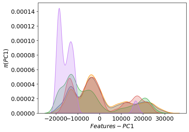
The distribution of the first principal component:

[26]:

%matplotlib inline
plots['dist_pc'][0]

[26]:

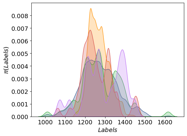
../_images/ipython_notebooks_active_model_based_41_0.png

The distribution of the labels:

[27]:

plots['dist_y'][0]

[27]:

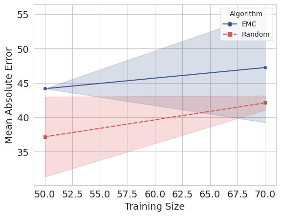
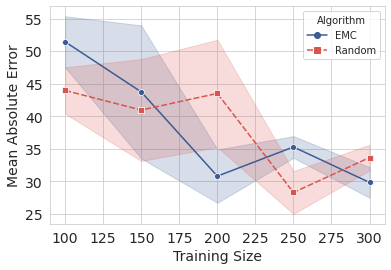
../_images/ipython_notebooks_active_model_based_43_0.png

The learning curves:

[28]:

plots['learning_curve']

[28]:

../_images/ipython_notebooks_active_model_based_45_0.png

Search in a loop

This is how we use this module in a loop:

[29]:

import os
warnings.filterwarnings('ignore')

out_dir = 'al_toy_example' # the arbitrary path to the output directory
if not os.path.exists(out_dir):
    os.makedirs(out_dir)

# all data sets must be 2-dimensional
y = density.values.reshape(-1,1)

al = ActiveLearning(
           model_creator = model_creator,
           U = features,
           target_layer = ['b1_l2', 'b2_l2'], # we could also enter 'merged' layer because it only does the concatenation
           train_size = 100,  # 100 initial training data will be selected randomly
           test_size = 50,  # 50 independent test data will be selected randomly for the entire search
           batch_size = [50,0,0] # at each round of AL, labels for 20 candidates will be queried using EMC method
           )

tr_ind, te_ind = al.initialize()


al.deposit(tr_ind, y[tr_ind])
al.deposit(te_ind, y[te_ind])


while al.query_number < 5:
    early_stopping = EarlyStopping(monitor='val_loss', min_delta=1e-6, patience=20, verbose=0, mode='auto')
    tr_ind = al.search(n_evaluation=3, ensemble='kfold', n_ensemble=3, normalize_input=True, normalize_internal=False,
    batch_size=32, epochs=5, verbose=0)#, callbacks=[early_stopping],validation_split=0.1)

    al.results.to_csv(out_dir+'/emc.csv',index=False)

    pd.DataFrame(al.train_indices).to_csv(out_dir+'/train_indices.csv',index=False)
    pd.DataFrame(al.test_indices).to_csv(out_dir+'/test_indices.csv',index=False)

    al.deposit(tr_ind, y[tr_ind])

    # you can run random search later but, I need it to be in my learning curve
    al.random_search(y, n_evaluation=3, random_state=13, batch_size=32, epochs=5, verbose=0)#, callbacks=[early_stopping],validation_split=0.05)

    al.random_results.to_csv(out_dir+'/random.csv',index=False)

    plots = al.visualize(y)
    if not os.path.exists(out_dir+"/plots"):
        os.makedirs(out_dir+"/plots")

    plots['dist_pc'][0].savefig(out_dir+"/plots/dist_pc_0_%i.png"%al.query_number , close = True, verbose = True)
    plots['dist_y'][0].savefig(out_dir+"/plots/dist_y_0_%i.png"%al.query_number , close = True, verbose = True)
    plots['learning_curve'].savefig(out_dir+"/plots/lcurve_%i.png"%al.query_number, close = True, verbose = True)

we stored 100 of passed indices. A list of them is in the 'last_deposited_indices_' attribute.
we stored 50 of passed indices. A list of them is in the 'last_deposited_indices_' attribute.
WARNING:tensorflow:6 out of the last 25 calls to <function Model.make_predict_function.<locals>.predict_function at 0x7f110b89c9d0> triggered tf.function retracing. Tracing is expensive and the excessive number of tracings could be due to (1) creating @tf.function repeatedly in a loop, (2) passing tensors with different shapes, (3) passing Python objects instead of tensors. For (1), please define your @tf.function outside of the loop. For (2), @tf.function has experimental_relax_shapes=True option that relaxes argument shapes that can avoid unnecessary retracing. For (3), please refer to https://www.tensorflow.org/guide/function#controlling_retracing and https://www.tensorflow.org/api_docs/python/tf/function for  more details.
we stored 50 of passed indices. A list of them is in the 'last_deposited_indices_' attribute.
WARNING:tensorflow:5 out of the last 23 calls to <function Model.make_predict_function.<locals>.predict_function at 0x7f10d81f3f70> triggered tf.function retracing. Tracing is expensive and the excessive number of tracings could be due to (1) creating @tf.function repeatedly in a loop, (2) passing tensors with different shapes, (3) passing Python objects instead of tensors. For (1), please define your @tf.function outside of the loop. For (2), @tf.function has experimental_relax_shapes=True option that relaxes argument shapes that can avoid unnecessary retracing. For (3), please refer to https://www.tensorflow.org/guide/function#controlling_retracing and https://www.tensorflow.org/api_docs/python/tf/function for  more details.
we stored 50 of passed indices. A list of them is in the 'last_deposited_indices_' attribute.
WARNING:tensorflow:5 out of the last 23 calls to <function Model.make_predict_function.<locals>.predict_function at 0x7f107c3d9ee0> triggered tf.function retracing. Tracing is expensive and the excessive number of tracings could be due to (1) creating @tf.function repeatedly in a loop, (2) passing tensors with different shapes, (3) passing Python objects instead of tensors. For (1), please define your @tf.function outside of the loop. For (2), @tf.function has experimental_relax_shapes=True option that relaxes argument shapes that can avoid unnecessary retracing. For (3), please refer to https://www.tensorflow.org/guide/function#controlling_retracing and https://www.tensorflow.org/api_docs/python/tf/function for  more details.
we stored 50 of passed indices. A list of them is in the 'last_deposited_indices_' attribute.
WARNING:tensorflow:5 out of the last 23 calls to <function Model.make_predict_function.<locals>.predict_function at 0x7f107c6bd550> triggered tf.function retracing. Tracing is expensive and the excessive number of tracings could be due to (1) creating @tf.function repeatedly in a loop, (2) passing tensors with different shapes, (3) passing Python objects instead of tensors. For (1), please define your @tf.function outside of the loop. For (2), @tf.function has experimental_relax_shapes=True option that relaxes argument shapes that can avoid unnecessary retracing. For (3), please refer to https://www.tensorflow.org/guide/function#controlling_retracing and https://www.tensorflow.org/api_docs/python/tf/function for  more details.
we stored 50 of passed indices. A list of them is in the 'last_deposited_indices_' attribute.
WARNING:tensorflow:5 out of the last 23 calls to <function Model.make_predict_function.<locals>.predict_function at 0x7f10d855a160> triggered tf.function retracing. Tracing is expensive and the excessive number of tracings could be due to (1) creating @tf.function repeatedly in a loop, (2) passing tensors with different shapes, (3) passing Python objects instead of tensors. For (1), please define your @tf.function outside of the loop. For (2), @tf.function has experimental_relax_shapes=True option that relaxes argument shapes that can avoid unnecessary retracing. For (3), please refer to https://www.tensorflow.org/guide/function#controlling_retracing and https://www.tensorflow.org/api_docs/python/tf/function for  more details.
we stored 50 of passed indices. A list of them is in the 'last_deposited_indices_' attribute.

[30]:

al.results

[30]:

	num_query	num_training	num_test	mae	mae_std	rmse	rmse_std	r2	r2_std
0	0	100	50	51.426883	3.928198	65.619069	3.901240	0.297333	0.084853
1	1	150	50	43.730914	10.224642	55.313881	13.132943	0.474416	0.255601
2	2	200	50	30.796186	4.091387	38.563045	4.048841	0.755510	0.052260
3	3	250	50	35.275099	1.672109	42.915425	1.183024	0.700281	0.016584
4	4	300	50	29.824896	3.473710	36.496102	5.330896	0.778783	0.065220

[31]:

al.random_results

[31]:

	num_query	num_training	num_test	mae	mae_std	rmse	rmse_std	r2	r2_std
0	0	100	50	43.952071	3.569051	56.381525	5.837295	0.477530	0.107432
1	1	150	50	40.947933	7.829895	51.703703	11.578128	0.543490	0.208759
2	2	200	50	43.502437	8.242243	55.426619	10.814782	0.481414	0.207281
3	3	250	50	28.283638	3.291657	35.423523	3.174839	0.794309	0.035551
4	4	300	50	33.646365	1.965678	42.593052	1.539270	0.704606	0.021051

[32]:

plots = al.visualize(y)
plots['learning_curve']

[32]:

../_images/ipython_notebooks_active_model_based_50_0.png

Create a video

If you store all the plots at each round you will be able to create a video similar to these ones:

[33]:

from IPython.display import HTML
from base64 import b64encode
with open("images/dist_y.mov", "rb") as f:
    video = f.read()
video_encoded = b64encode(video).decode('ascii')
video_tag = '<video controls alt="test" src="data:video/x-m4v;base64,{0}">'.format(video_encoded)
HTML(data=video_tag)

[33]:

[34]:

from IPython.display import HTML
from base64 import b64encode
with open("images/lcurve.mov", "rb") as f:
    video = f.read()
video_encoded = b64encode(video).decode('ascii')
video_tag = '<video controls alt="test" src="data:video/x-m4v;base64,{0}">'.format(video_encoded)
HTML(data=video_tag)

[34]: